When giving my first presentation at an international conference as a young postgraduate, I was asked some tough questions about my work. The critique certainly had its merits, but the tone was a little harsh. The professor — I was told afterwards — was a believer in trial by fire, that is, testing the students under pressure. I didn’t mind it that much, but the organizers went on to hold a meeting to lay down some ground rules for the following sessions. Anyway, as I was about to step down from the podium I managed to respond: “Like Rosenblatt said, one learns only from mistakes”. What a silly thing to say!

Although my response was merely an attempt to brush off the humiliation, there was a grain of truth in it – at least with respect to the computational theory of mind. Its main idea is that although human mind is not a computer as such, it processes information along the same principles as modern digital computers.

Frank Rosenblatt (1928-1971) was one of the pioneers of the artificial intelligence. In 1958 he presented an idea of Perceptron, an algorithm that showed the elementary capability of learning and storing knowledge. The device Rosenblatt built for the U.S. Navy could be taught to, for instance, recognize basic geometric shapes.

Basically, the perceptron was a simple linear classifier based on the model of artificial neurons developed by Warren McCullough and Walter Pitts in 1943. As illustrated below, the neuron receives an input signal x composed of n values. It does some computation and outputs the result y that represents a binary decision, yes or no.

The input values could be the values of pixels in an image (e.g., character recognition), the occurences of certain words in a piece of text (e.g., spam detection), or readings from some physical tests (e.g., diagnosis). The output value y represents a decision ”yes, it is a C”, ”no, it is not spam”, or ”yes, there is a risk of heart a disease”. Essentially, a neuron can be taught to recognize one concept: whether some signal is the of concept type (a character, a spam email, a case of heart disease) or not.

Perceptron has a weight w associated with each input x representing the relative importance of each input with respect to the taught concept. For instance, in the case of spam detection, the presence of words like win, money, and special are likely to be more important than words like, say, escalator, and hence their weights are likely to be higher. In addition to weights, Perceptron has a threshold value or bias to gauge the output.

One can view the input signal is a n-dimensional vector, and the weights as another n-dimensional vector. The decision can be expressed in terms linear algebra: a linear function f(x) that is an inner-product of the signal and the weights plus the bias:

The result of f(x) is still a real-value, not a decision. In the above illustration, the function φ(v) translates the real-value into a decision: If f(x) > 0, then the decision is 1 (positive), otherwise -1 (negative).

The weight vector and the bias form a hyperplane that divides the n-dimensional space of input signals into two parts. The illustration below shows a two-dimensional space with red and blue dots separated by a hyperplane defined by weights w and bias b. The weights form the normal of the hyperplane, and bias varies the distance from the origin, respectively. 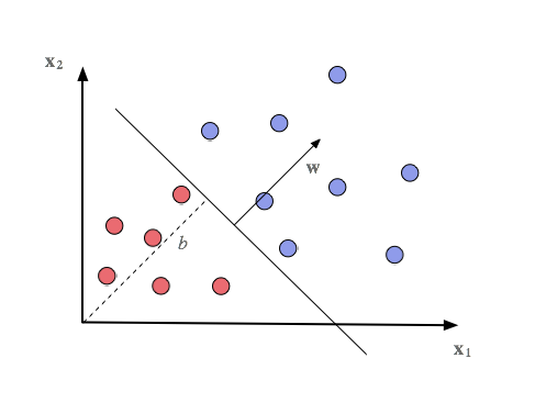The function f(x) measures the distance from a dot to the hyperplane. If the outcome is positive, the decision is yes, if zero or negative, no. All possible input signals (dots) are on one side of the hyperplane or on the other. That’s a dichotomy if there ever was one.

How does one figure out the weights? This is where one learns only from mistakes. Training is done presenting the perceptron a set of signals accompanied with labels. In other words, to learn to recognize spam, the perceptron could be trained with 1,000 samples of spam emails and 5,000 or 10,000 samples normal emails — the numbers should represent the actual frequency of the concept.

So, one presents the data one-by-one to the perceptron and compares output to the accompanied label. If they are the same, all is good. If they are not, then the perceptron has made an error and the weights have to be adjusted. The adjustments are made in small steps, and the whole training data is run through the perceptron multiple times. Each run of the complete training data is called an epoch.

Over the years, I have written perceptrons in various languages, but this is my first attempt at it with Scala. It is a functional programming language that encourages referential transparency, i.e., that all effects of a function are in the return value. Typically, one uses read-only variables and resorts to recursion for iteration, for instance.

The whole source code can be found on GitHub, but I’ll post some of the juicy parts here. First, we have two data structures: one for labeled samples composed of input signals and a label (1 for positives and -1 for negatives), and another for the weight vector and the bias.

case class LabeledSample(x: Array[Double], label: Int)
case class Weights(w: Array[Double], b: Double)

The trainer itself has two variables: the learning rate eta or η for tuning how coarse and fast or how refined and slow the training should be, and the maximum number of epochs we will run.

class LinearPerceptronTrainer(eta: Double, epochs: Int)

The training epochs are run in a tail recursive loop. Each trial adjusts the weights for the next trial. Each epoch produces new weights and the number of errors it yields on the training data. Should it commit no classification errors, we’ll stop.

In addition to learning rate, we use radius (r in the snippet below) as a guide in adjusting the bias. The radius is simply the length of the longest vector in the training data. The idea was adopted from Christianini & Shawe-Taylor (2000). Naturally, there are other ways to go about adjusting the bias.

@tailrec
final def iterate(epoch: Int, data: List[LabeledSample],
  weights: Weights, r: Double): (Weights, Int) = {
  val (adjWeights, errors) = trial(data, weights, r)
  if (epoch == 0 || errors == 0) {
    (adjWeights, errors)
  } else {
    iterate(epoch - 1, data, adjWeights, r)
  }
}

After all this delegation, the actual learning takes place during the single run of the data. Scala’s foldLeft-operation enables us to iterate through data and accumulate (into acc) the changes resulting from each error. So the outcome of the whole foldLeft is the adjusted weights and the associated number of errors.

First, we calculate the inner product between the sample vector (signal input) and the current weight vector. If the inner product agrees with the label we continue on, but if they disagree, i.e., are of different sign, one positive and one negative, we adjust the weights.

def trial(data: List[LabeledSample],
  weights: Weights, r: Double): (Weights, Int) = {
  data.foldLeft(weights, 0) { (acc, s) =>
    val p = innerProduct(s.x, weights.w) + weights.b
    if (p * s.label <= 0) {
      (Weights(
        acc._1.w.zip(s.x). // pair weights and samples (inputs)
        map(w => w._1 + eta * s.label * w._2), // adjust weights
        acc._1.b + (eta * s.label * r * r)),   // adjust bias
        acc._2 + 1)                            // adjust errors
    } else {
      acc
    }
  }
}

At first glance, the adjustment phase may appear a bit messy. (I’ve named the fields and variables with short and convenient code snippets in mind rather than good practice. I’m not sure it has been a good decision.) Effectively, it produces a pair of Weights object and the error count. The zip operation merely pairs the elements of two lists so they can be processed in one go. The adjustment of the weights reads

where w_{t + 1} is the adjusted weights, w_t the current weights, η is the learning rate, y_i the ith sample label and x_i the ith sample vector in the data. In a similar vein, the adjustment of the bias can be expressed as

where b_{t + 1} is the new bias, b_t the current bias, and R the radius.

We’ll test it with a small mock dataset.

val data = List(
  LabeledSample(Array[Double](0.0d, 2.0d), -1),
  LabeledSample(Array[Double](1.0d, 2.0d), -1),
  LabeledSample(Array[Double](2.0d, 1.0d), -1),
  LabeledSample(Array[Double](2.0d, 5.0d), 1),
  LabeledSample(Array[Double](3.0d, 3.0d), 1),
  LabeledSample(Array[Double](4.0d, 3.0d), 1)
)

We’ll start with zero weight vector and zero bias. The learning rate is set to 0.001. The training runs for eight epochs as follows:

epoch 1 : (w: [0.0,0.0], b: 0.0, errors: 6)
epoch 2 : (w: [0.006,0.006], b: 0.0, errors: 3)
epoch 3 : (w: [0.003,0.001], b: -0.087], errors: 3)
epoch 4 : (w: [0.012,0.012], b: 0.0], errors: 3)
epoch 5 : (w: [0.009,0.007], b: -0 .087], errors: 3)
epoch 6 : (w: [0.018,0.018], b: 0.0], errors: 3)
epoch 7 : (w: [0.014,0.013], b: -0.087], errors: 1)
epoch 8 : (w: [0.018,0.016], b: -0.058], errors: 0)
Finished in 31 ms (w: [0.018,0.016], b: -0.058], errors: 0)

So, there it is. The weight vector and bias are trained to recognize a mock concept in a two-dimensional space. The learning process is error-driven, i.e., it learns only from mistakes. There is a wisp of generalization (however meager): instead of the actual samples, the model contains a derived hyperplane that applies to all input signals instead of just those it has encountered. Some have animated the progress of Perceptron training using larger data.

Perceptron is certainly not a state-of-the-art classifier. However, from this simple classifier, I hope to make casual excursions into related topics, various other classifiers and classification problems. And whatever comes to mind.

Further reading:

• Christianini, Nello and Shawe-Taylor, John (2000), Introduction to Support Vector Machines and other kernel-based learning methods. Cambridge University Press, Cambridge, UK.
• Rosenblatt, Frank (1958), The Perceptron: A Probabilistic Model for Information Storage and Organization in the Brain, Cornell Aeronautical Laboratory, Psychological Review, 65(6), 386–408.

The LaTeX-snippets were created with CodeCogs online editor. The source code can be found in GitHub.